The Navier-Stokes equations describe the motion of Newtonian fluids. This equation provide a complete model for fluid motion, capturing pressure, viscosity, and external forces, helpful for analysing real-world engineering problems like designing dams, aircraft, ocean currents, water flow in a pipe, blood flow in arteries or predicting weather in India.
In this article, we will discuss
- Introduction
What is need of introducing Navier-stokes equation if we have simpler equation like Euler, Bernoulli's equation etc.
Derivation of Navier-stokes theorem- Derivation of other equation from Navier-Stokes Theorem
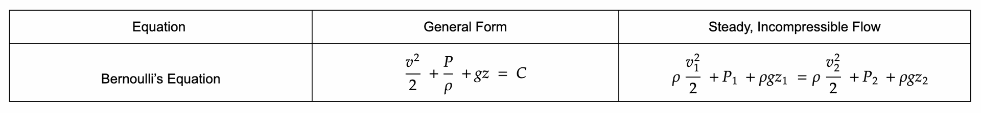
Bernoulli's equation
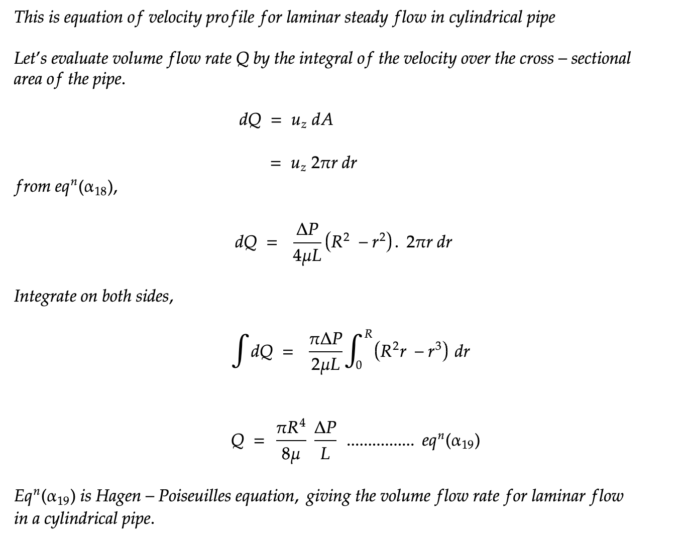
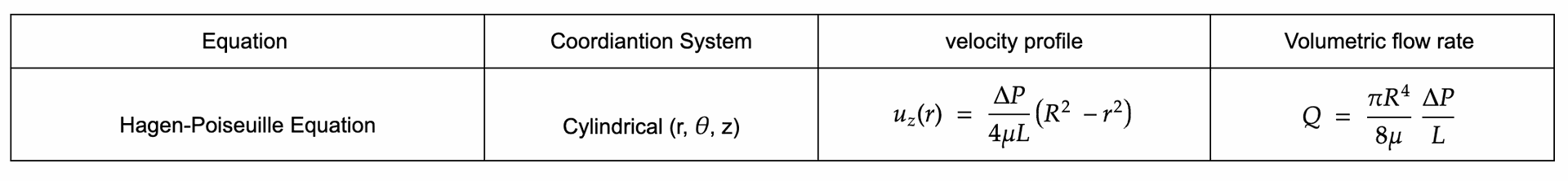
Hagen-Poiseuille's equation
Euler's Equation- Case Study: Modeling Cyclone Turbulence with Navier-Stokes (Fani Cyclone in 2019 and Yaas Cyclone in 2021)
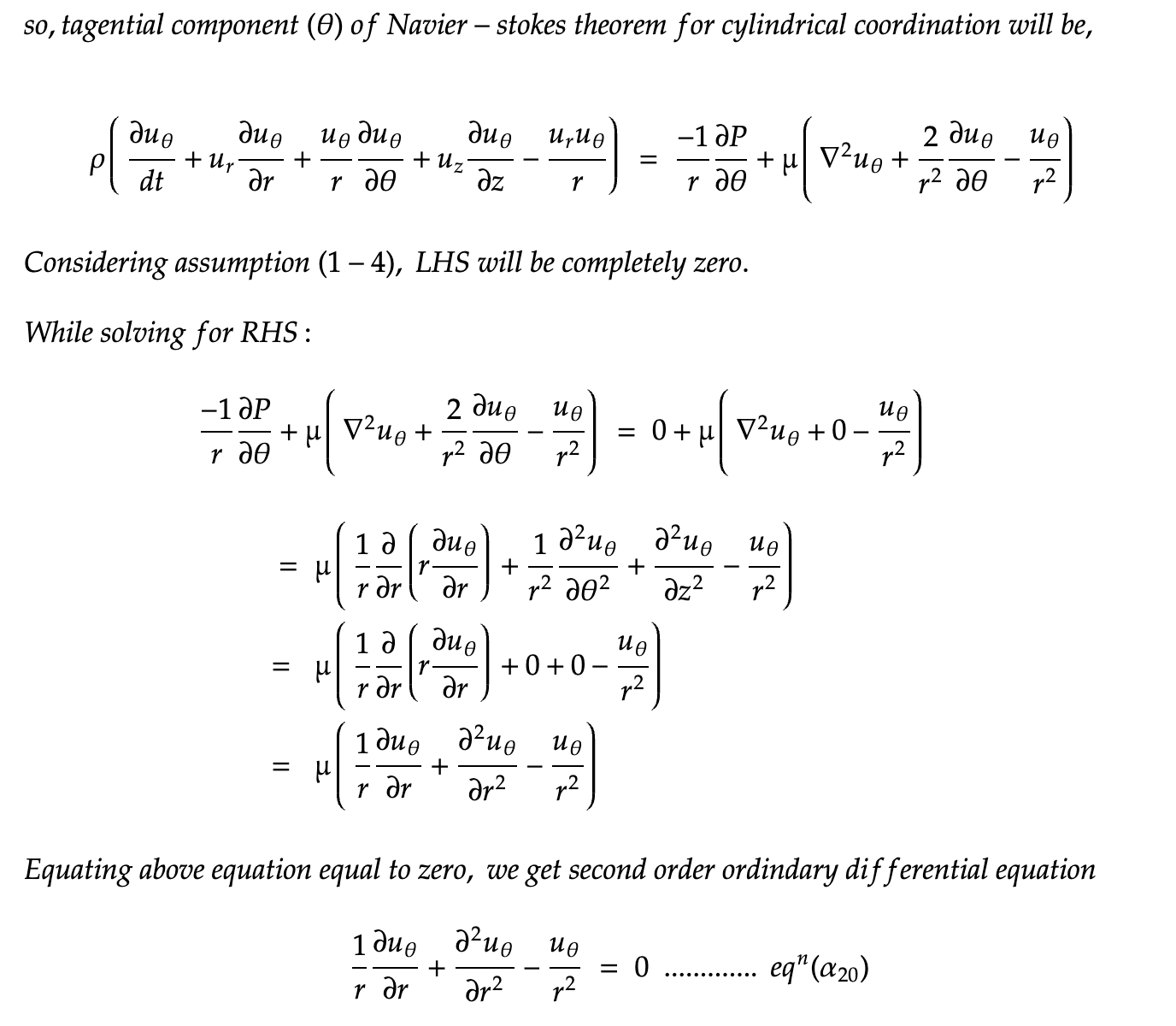
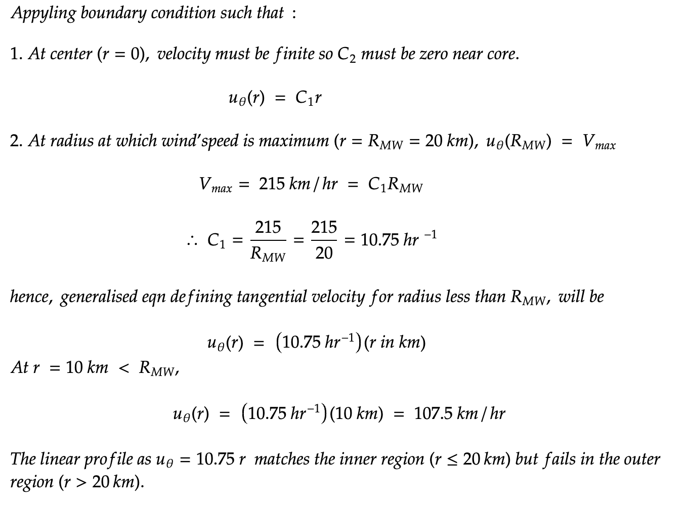
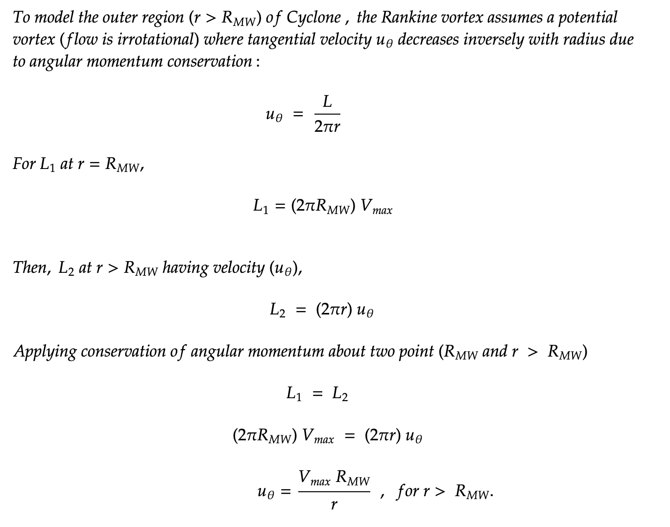
Evaluating tangential velocity and graphical representation
Calculating pressure drop and turbulence corrections- Summary Table
1. Introduction
- Negligence of Viscosity: Bernoulli's and Euler equation ignores viscous effects and friction losses, which can't be neglected in case of real flow such as friction in pipes, drag on car, air flowing over a aircraft wing. While Navier-Stokes (via Poiseuille’s law) gives the exact velocity profile, considering viscous effect in real fluid.
- Turbulence and Unsteady flow: Simpler equation like Bernoulli equation is linear equation defined for inviscid steady flow, fail to explain turbulence and unsteady flow due to their non-linearity nature (eg. monsoon winds) . So, convective term (u⋅∇)u in Navier-Stokes is nonlinear, allowing it to model complex phenomena like turbulence.
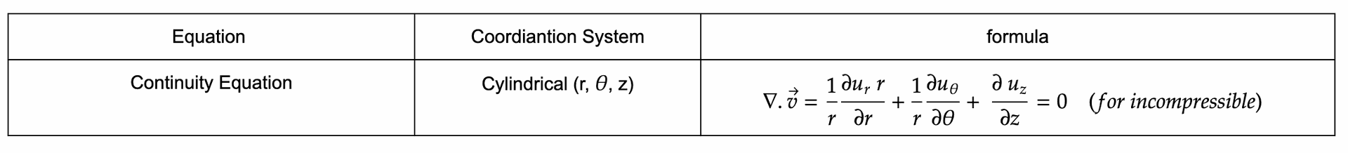
- Lack of momentum balance in Continuity Equation: The continuity equation (∇⋅u=0 for incompressible flow) ensures mass conservation but lack information about momentum balance. While Navier-Stokes combines continuity with momentum conservation for a complete description of fluid motion.
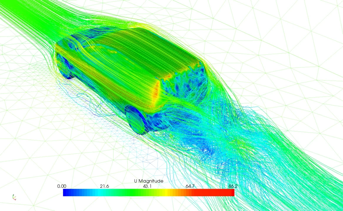
The Navier-Stokes equations tells us about how fluids (liquids and gases) move by applying Newton’s second law (F = ma) to a fluid element where F here is net force. We studied various force acting on fluid, mainly force due to pressure, viscosity (internal friction within fluid), and external force (gravity).
Let’s derive them step-by-step.
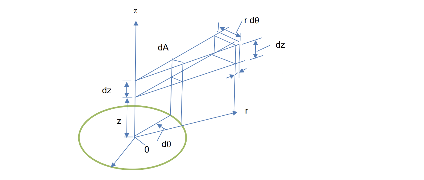
Step 1 : Taking Element and define properties
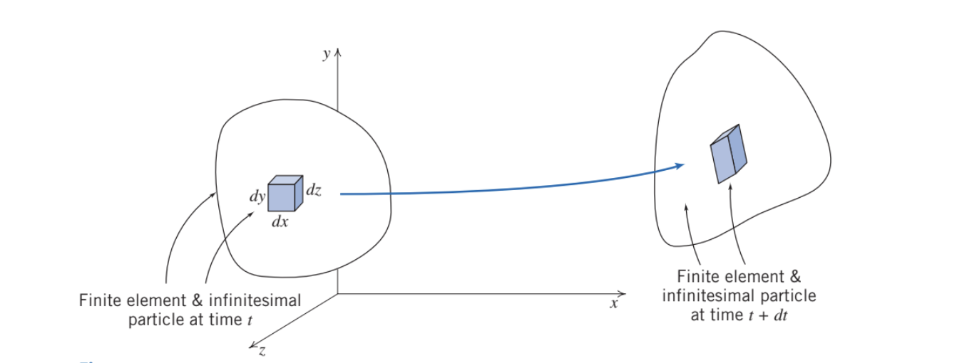
Imagine a tiny cube of fluid (like a small drop of water) moving in a river. Depending on its density and volume, mass of tiny fluid will be

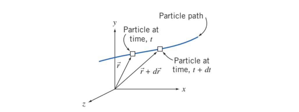
For moving fluid, we can define velocity in form of vector in x,y,z direction such that,

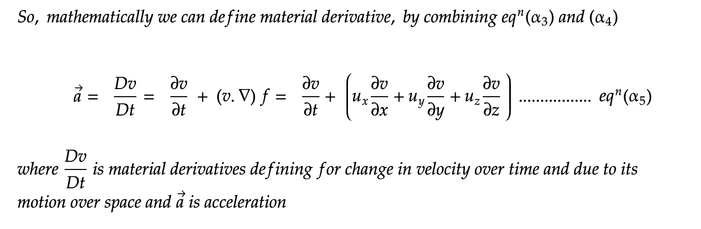
Also, rate of change of velocity with time and due to motion of fluid is related to acceleration. For such type of variation, we can a defined material derivatives.
Step 2: Defining material derivative for moving fluid
Now, you might be wondering what is material derivatives and how its different from other type of derivates such as ordinary and partial derivatives. Material derivative is a specific kind of total derivatives and it's unique as it is defined for moving fluid only.
The material derivative describes how a property of a fluid particle (like velocity, temperature, or density) changes as it moves through space and time such that:
- Changes in the property over time at a fixed point (local change).

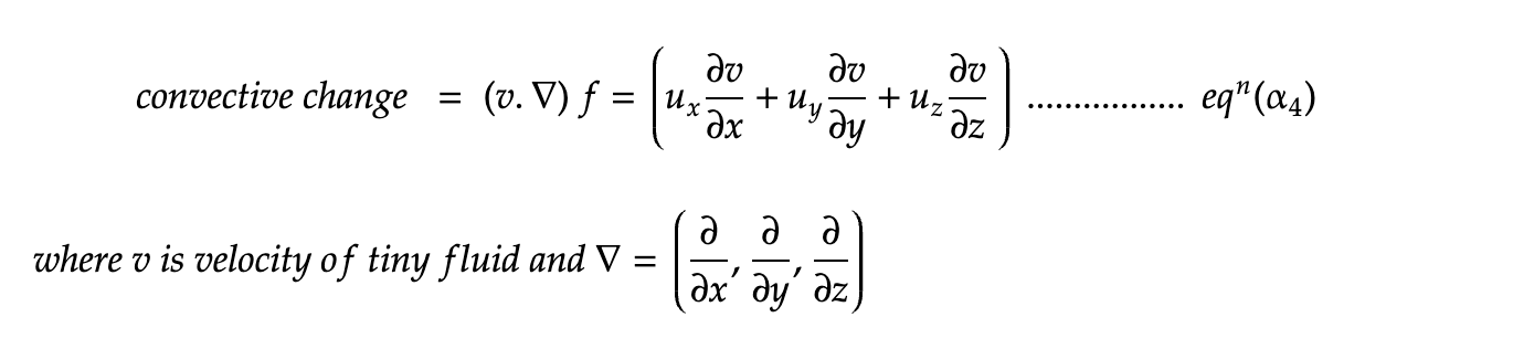
- Changes in the property due to the particle moving to a new location where conditions are different (convective change).
Imagine you’re tracking a specific drop of water in a river:
- If the river’s speed changes over time at your spot (e.g., due to a dam opening), that’s the ∂v/∂t part—local change.
- If the drop moves to a faster or slower part of the river (e.g., from calm water to rapids), that’s the convective part —change due to motion. The material derivative combines both to tell you how the drop’s velocity changes as it flows.
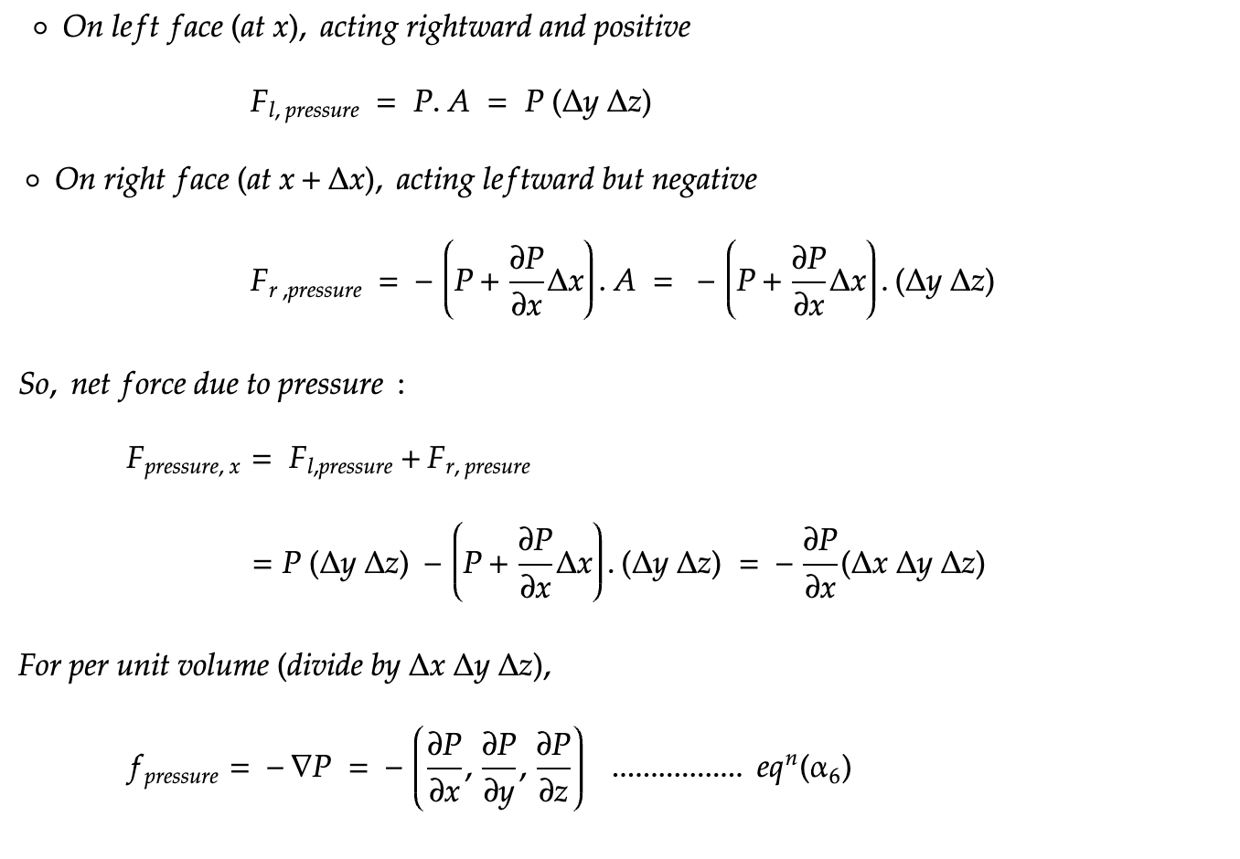
Step 3 : Evaluating force due to pressure
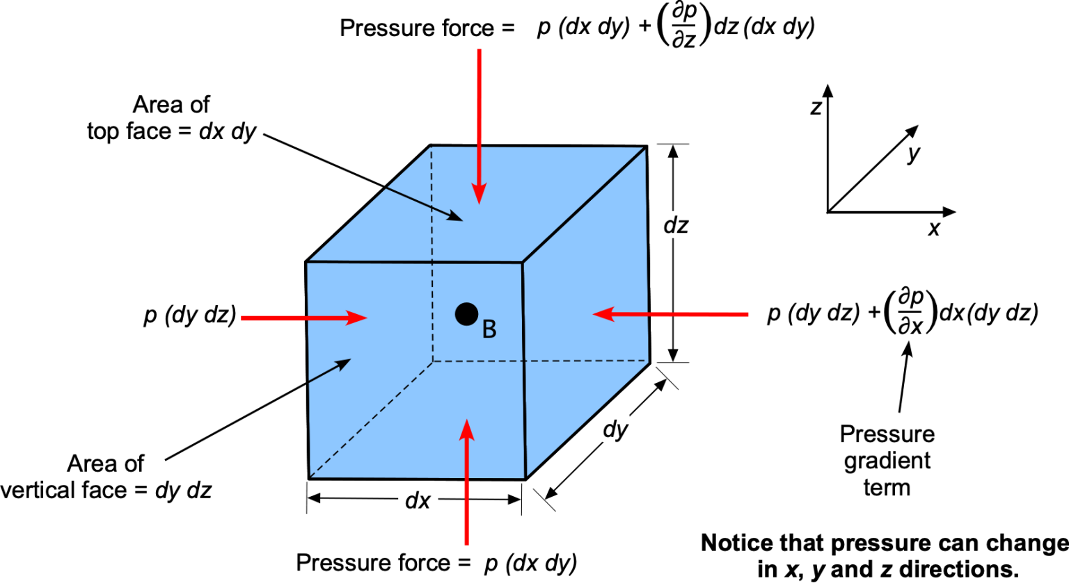
Pressure (P) pushes on the faces of the cube. For x-direction,
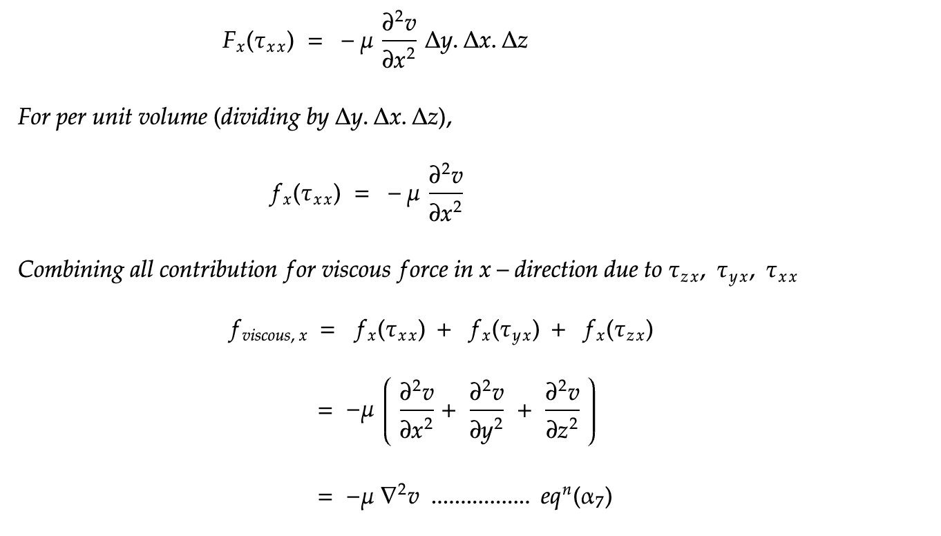
Step 4 : Viscous force (second contributing force)
Viscosity (μ) is like internal friction in the fluid. Viscosity arises from the interactions between molecules in a fluid, where stronger intermolecular forces lead to higher viscosity. A fluid with high viscosity will flow more slowly than a fluid with low viscosity when the same viscous force is applied.
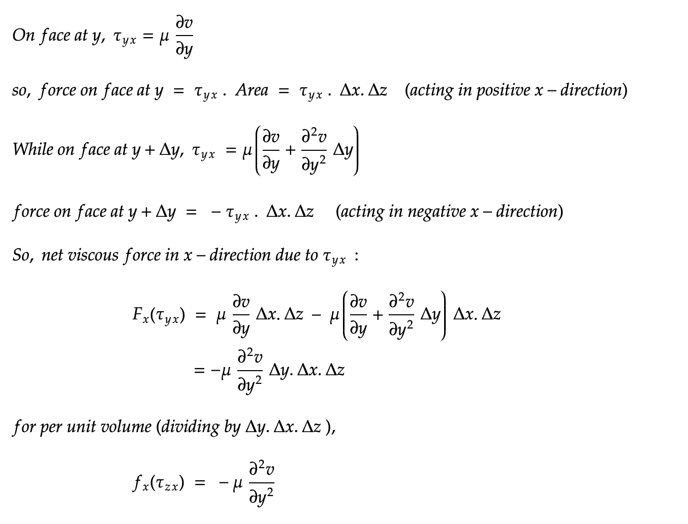
So, it causes shear stresses. For the x-direction, stress on the cube depends on how v (velocity) changes in y and z directions (shear) : τyx and τzx and x-direction (normal stress).
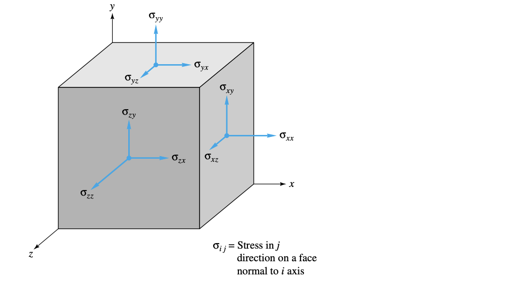
Consider the shear stress τyx (force in the x-direction on a face perpendicular to y):
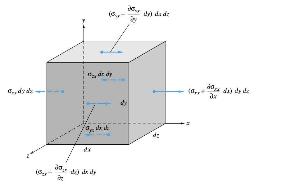
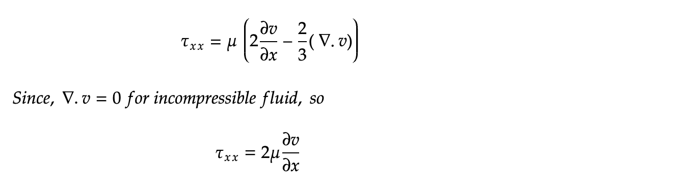
For normal viscous stress in the x-direction (τxx):
Net viscous force in x-direction due to τxx on faces at x and x+Δx will be,
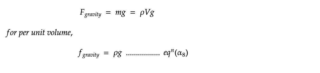
Step 5 : External Force (body force)
For external force, consider force due to gravity acting on tiny fluid,
Step 6 : Applying 2nd Newton law of force
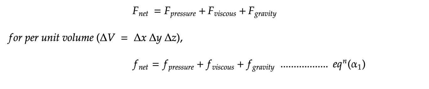
Newton’s second law states that the net force (F) acting on a body (or fluid element in this case) equals its mass (m) times its acceleration (a):
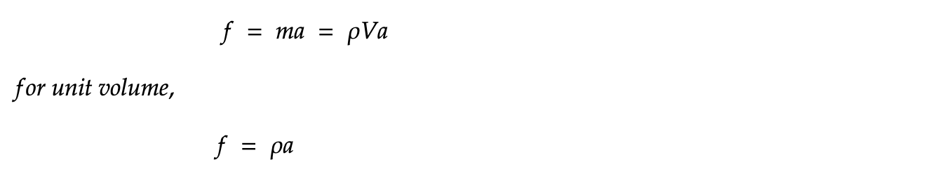
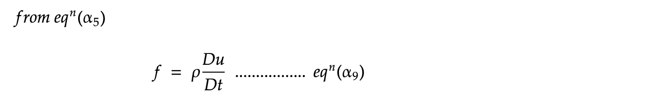
As earlier we have discussed that rate of change of velocity equal to acceleration is defined by a parameter, called as material derivative for moving fluid only over time and space due to variation in fluid motion.
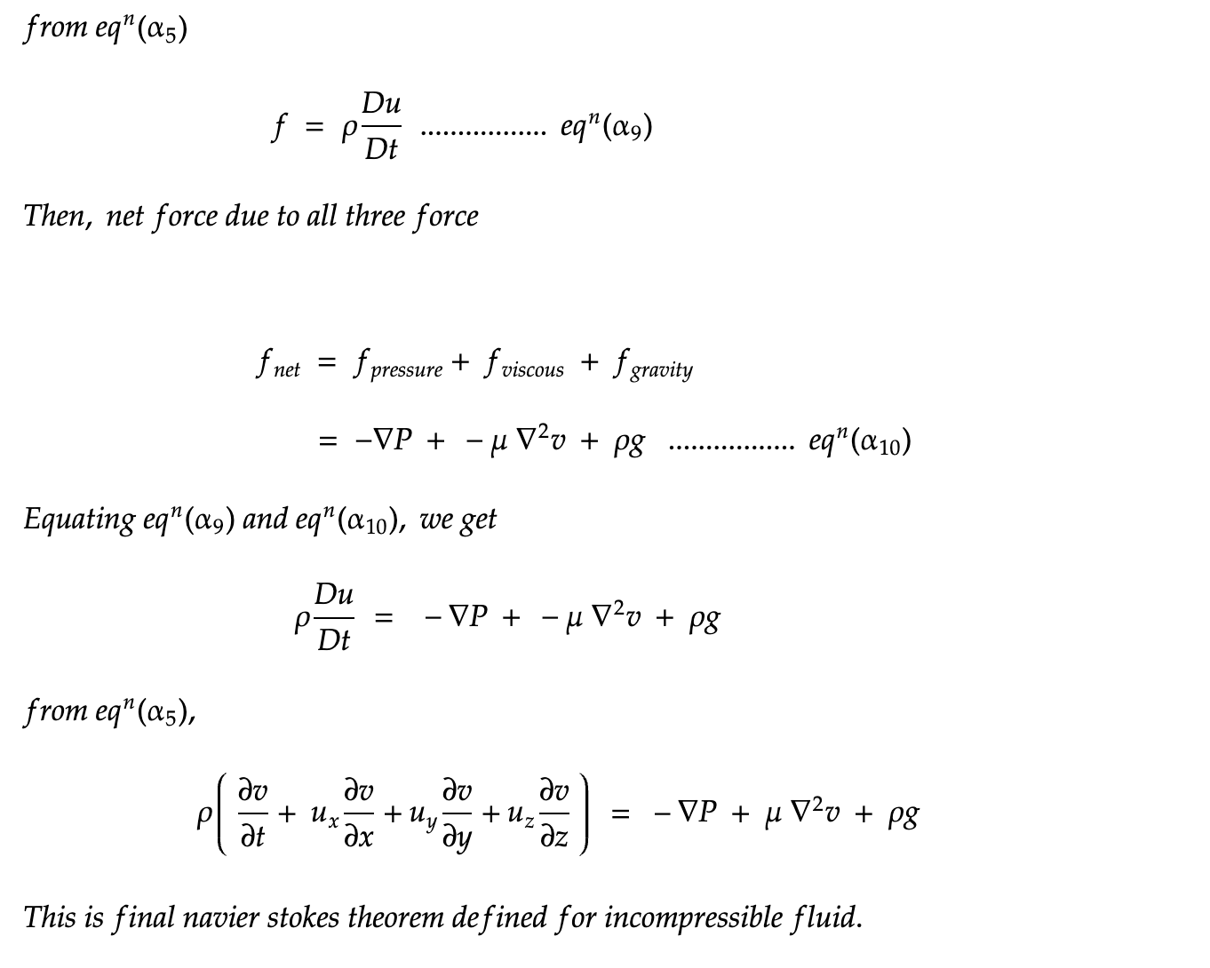
Also, net force on tiny fluid due to contribution of all three force, will be
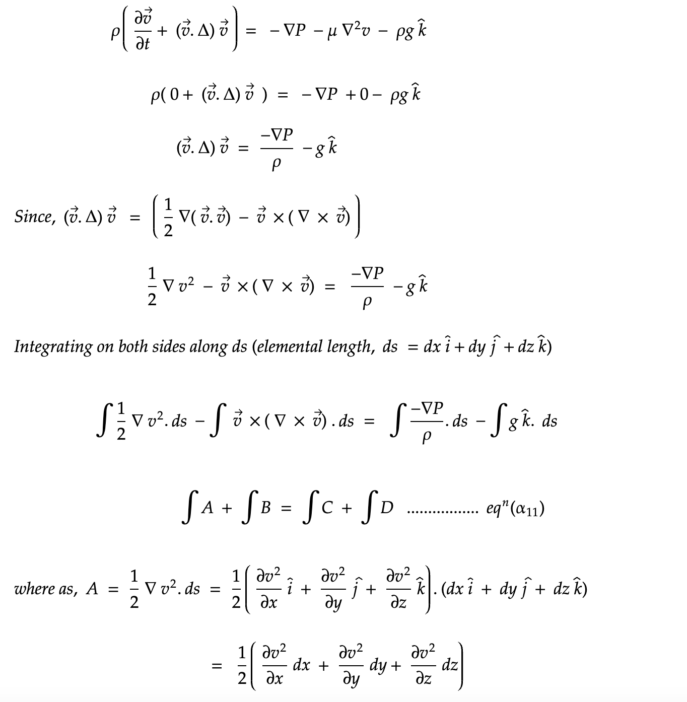
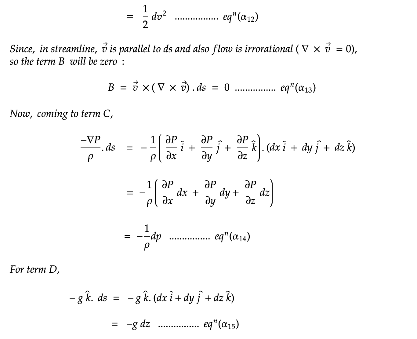
a. Bernoulli’s Equation (Inviscid, Steady Flow) :
Assumptions:
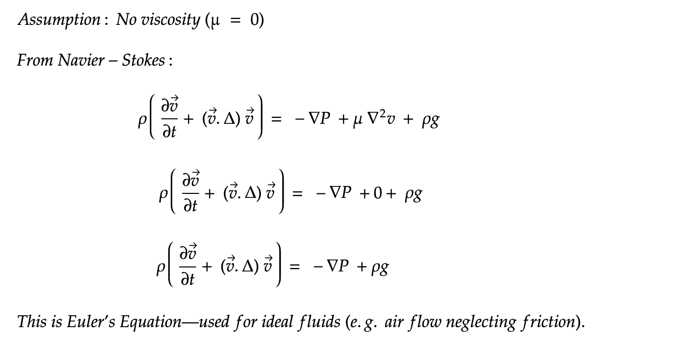
- Inviscid (μ = 0, no viscosity).
- Steady flow (∂v/∂t=0).
- Incompressible (∇⋅u=0).
- Along a streamline (no external forces perpendicular to flow).
- a downward force due to gravity in negative z-direction
Now, writing Navier-stokes theorem :

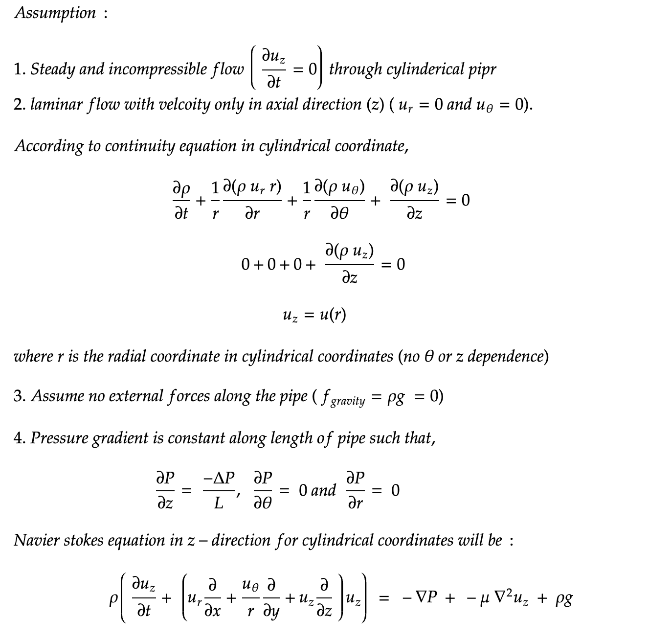
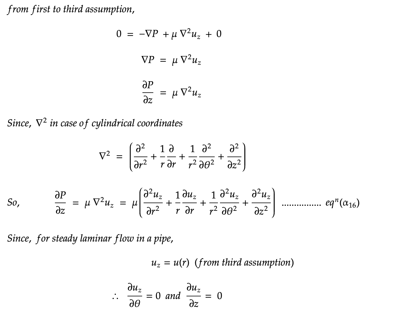
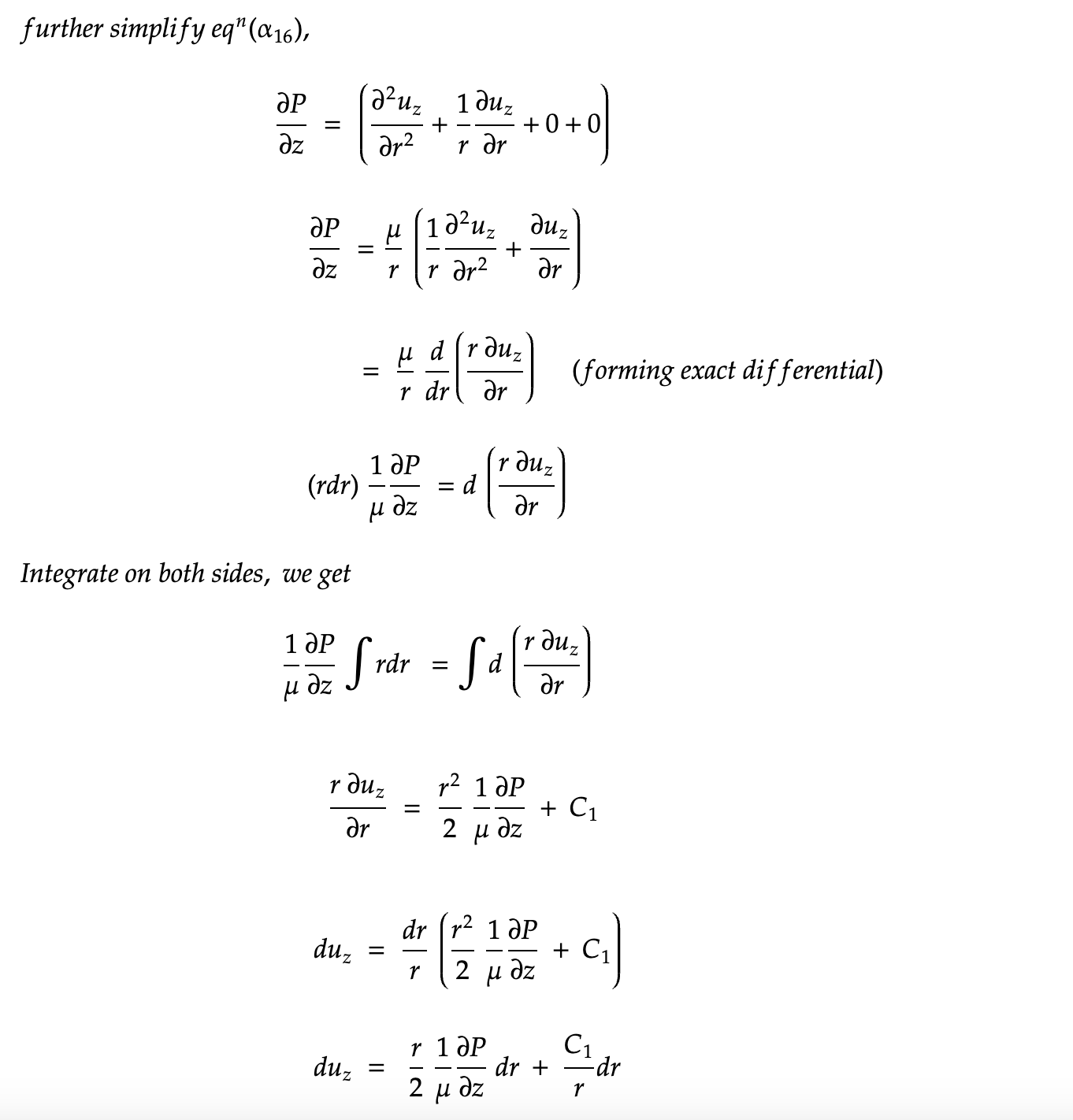
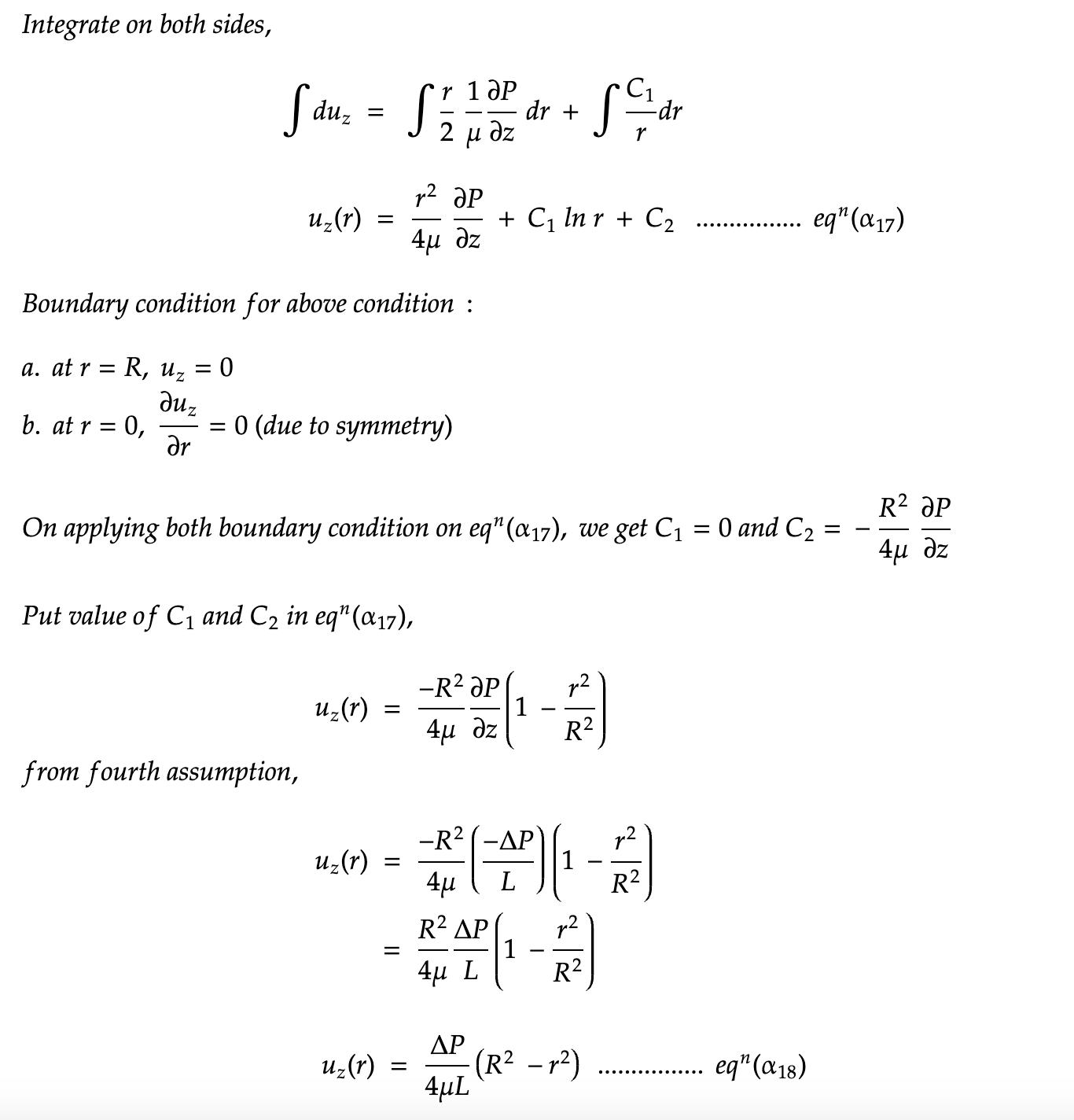
b. Poiseuille’s Law (Laminar Flow in a Pipe) :
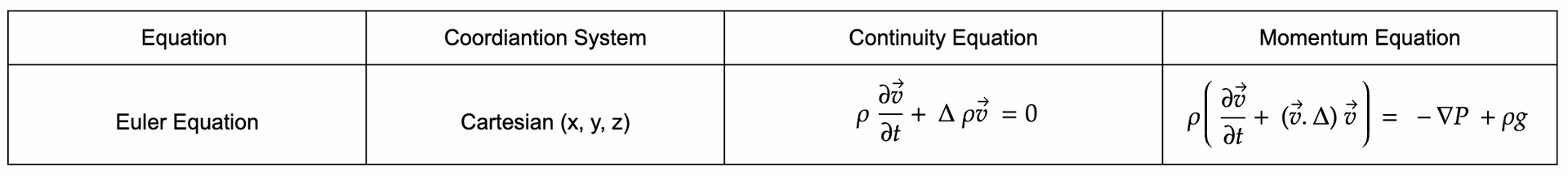
c. Euler’s Equation (Inviscid Flow)
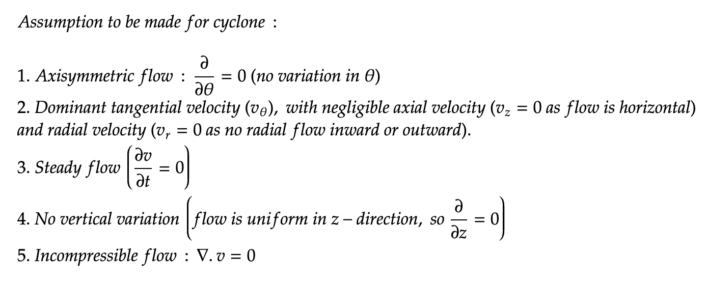
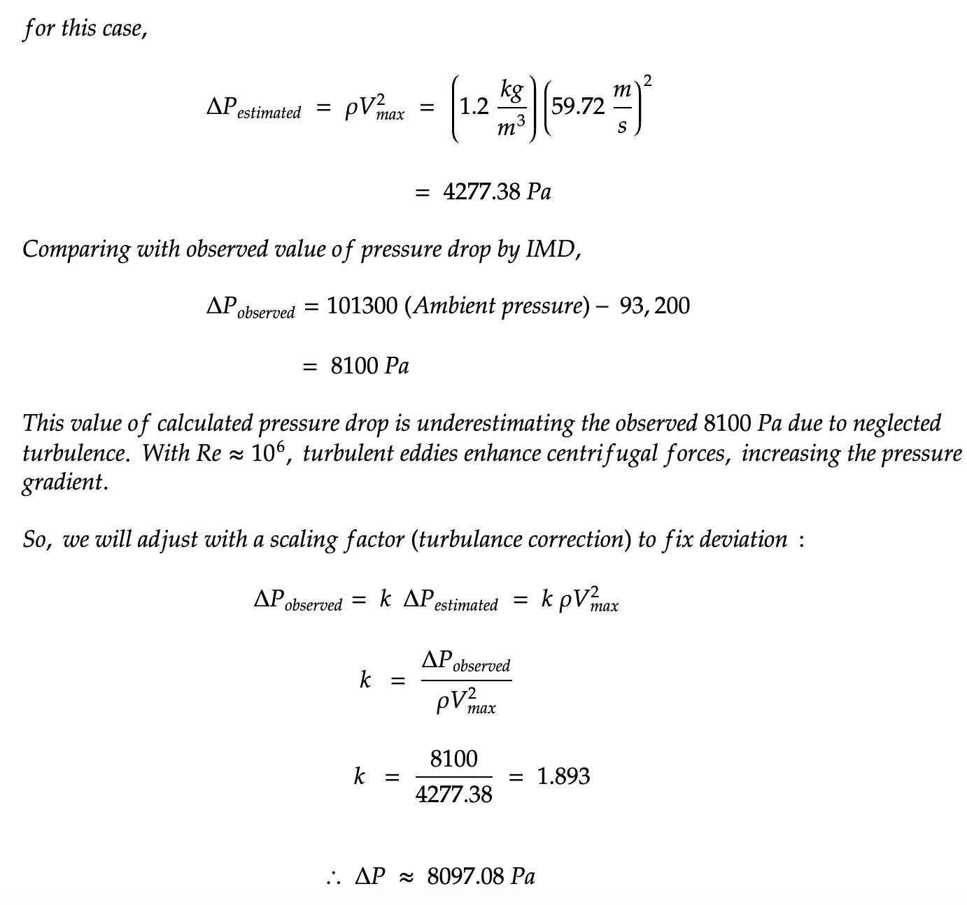
In India, cyclones like Fani (2019) and Yaas (2021) cause significant damage, making accurate prediction crucial. The Navier-Stokes equations model turbulent flow in cyclones by considering pressure gradients, viscosity, and nonlinear effects. For instance, in Cyclone Fani, the equations predict wind speeds of 200 km/h near the eyewall by solving for radial and tangential velocities in cylindrical coordinates, capturing three-dimensional turbulence (Reynolds number ~10^6).
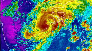
In contrast, Bernoulli’s equation, which assumes inviscid, steady flow, underestimates peak winds (e.g., predicting ~18 m/s vs. actual 59.72 m/s) and ignores turbulence and viscosity, making it inadequate for cyclone modeling. Navier-Stokes’ ability to handle complex, unsteady flows makes it essential for disaster management in India.
Official data for Cyclone Fani (2019) given by IMD (India Meteorological Department)
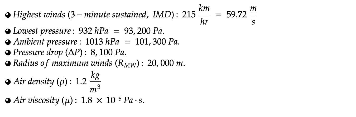

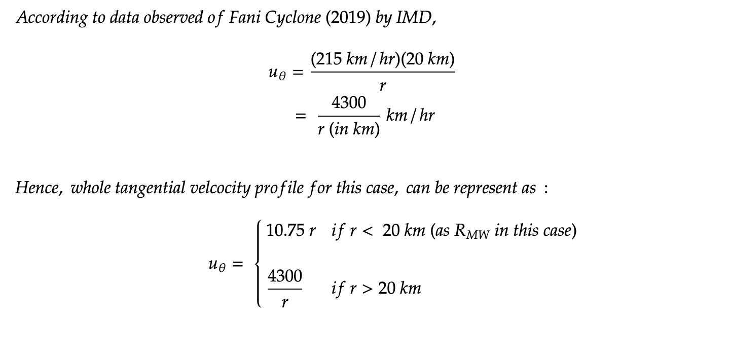
Graphical representation of tangential velocity with radius :
The tangential velocity profile of Cyclone Fani 2019 is plotted below, with radius r (km) on the x-axis (0 to 100 km) and tangential velocity uθ (km/h) on the y-axis (0 to 250 km/h).
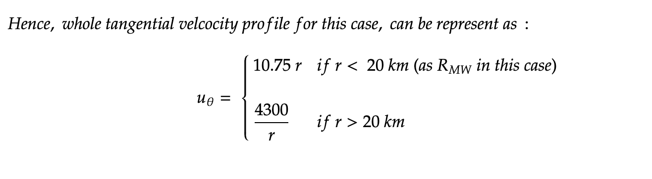
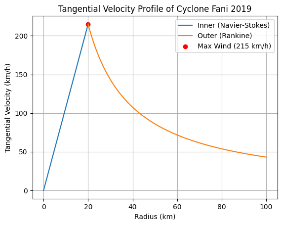
The red dot at (20, 215) highlights the observed maximum wind speed. At line of maximum wind speed, we can the transition from solid-body rotation (navier-stokes inner profile) to potential vortex flow (Rankine outer decay), to be consistent with meteorological observations.
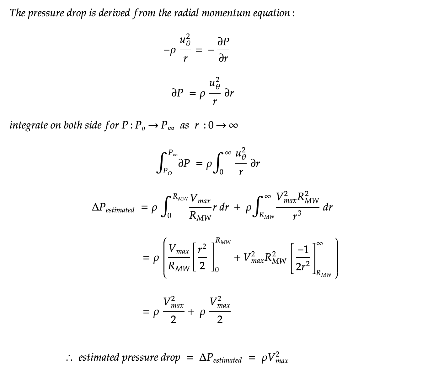
Calculating pressure drop and turbulence correction :
Summary Table
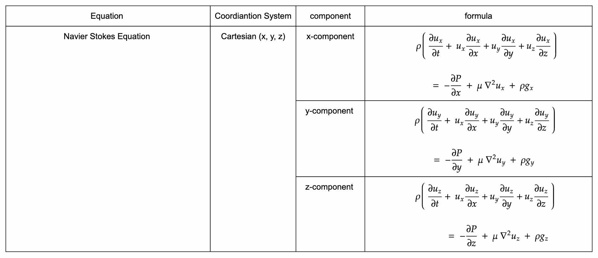
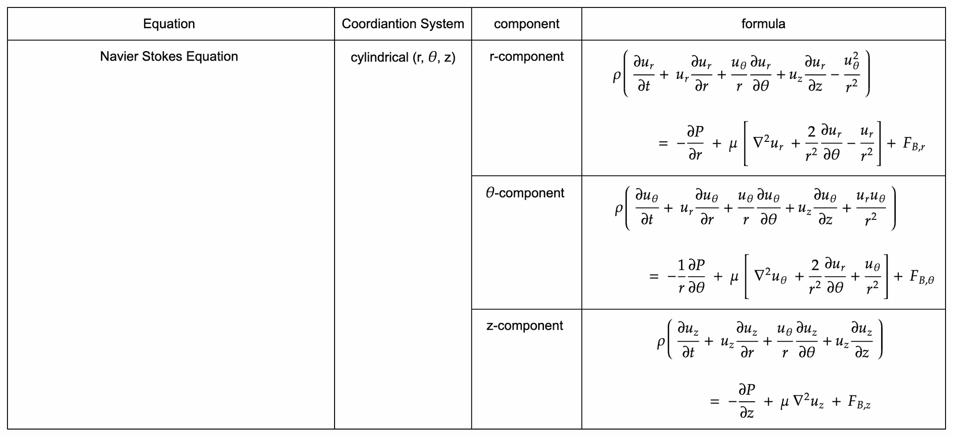


Navier Stokes Theorem